Working with rigid transmission line

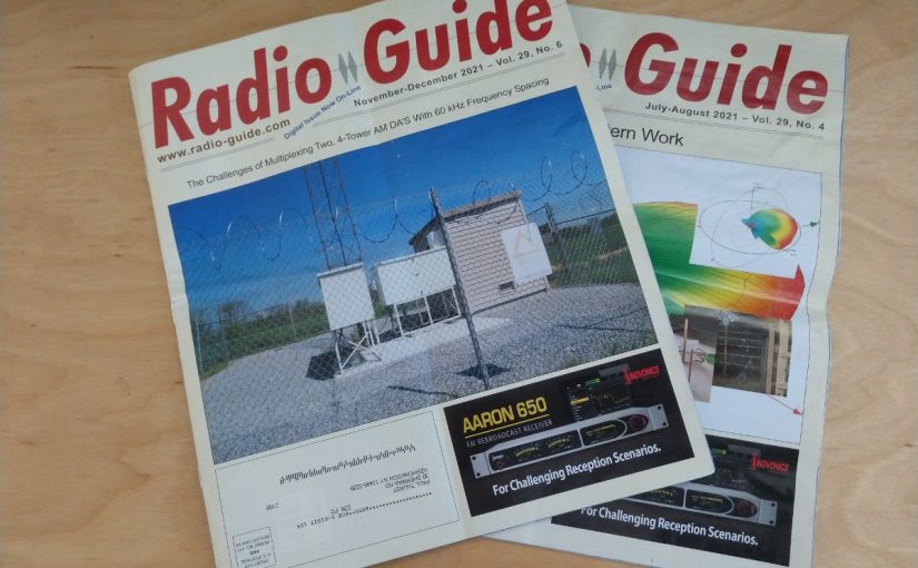
Update: This post is from several years ago (January 31, 2018), however, I did a fairly major revision and added a lot of information, so I am bumping it to the top of the pile. The header picture is from the Myat facility in Mahwah, New Jersey.

Installing transmitters requires a multitude of skills; understanding the electrical code, basic wiring, RF theory, and even aesthetics play some part in a good installation.  Working with rigid transmission line is a bit like working with plumbing (and is often called that). Rigid transmission line is often used within the transmitter plant to connect to a four-port coax switch, test load, backup transmitter, and so on.  Sometimes it is used outside to go up the tower to the antenna, however, such use has been mostly supplanted by Heliax-type flexible coax.

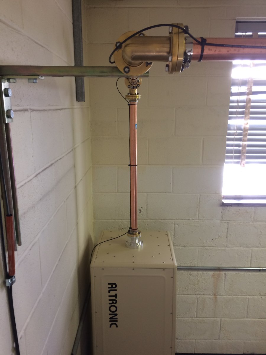
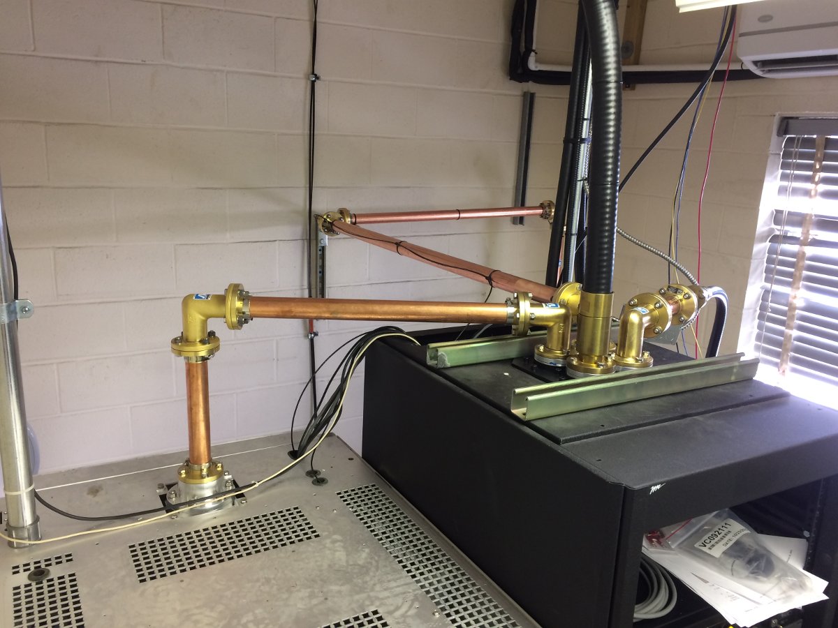
We completed a moderate upgrade to a station in Albany; installing a coax switch, test load, and backup transmitter.  I thought it would be interesting to document the rigid line work required to complete this installation.  The TPO at this installation is about 5.5 KW including the HD carriers.  The backup transmitter is a Nautel VS-1, analog only.

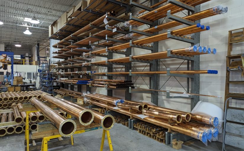
This site uses a 1 5/8-inch transmission line.  That line is good for most FM installations up to about 10-15 Kilowatts TPO.  Beyond that, 3-inch line should be used for TPOs up to about 30 Kilowatts. Above 30 KW TPO, 4 inch or greater line is required. There are a few combined FM stations that are pumping 80 or 90 KW up to the antenna. Those require 6 inch or greater line.  Even though the transmission lines themselves are rated to handle much more power, reflected power often creates nodes along the line where the forward power and reflected power are in phase.  This can create hot spots and if the reflected power gets high enough, flashovers.

This brings up another point; most rigid line comes in 20-foot sections. There are certain FM frequencies that require different lengths due to the aforementioned nodes that fall along the 1 wavelength intervals. If one of those nodes happens on a flange, that could create problems.

  • Frequencies between 88.1 and 95.9 MHz, use 20-foot line sections
  • Frequencies between 96.1 and 98.3 MHz, use 19.5-foot line sections
  • Frequencies between 98.5 and 100.1 MHz, use 19-foot line sections
  • Frequencies between 100.3 and 107.9 MHz, use 20-foot line sections

TV frequencies are much more complicated. The large channel width and much larger spectrum use means that close attention needs to be paid to line section length. Since low-power TV and translators may need to change frequency, those stations often use Heliax instead of rigid line.

Milwaukee portable band saw

Working with rigid line requires a little bit of patience, careful measurements, and some special tools.  Since the line itself is expensive and the transmission line lengthener has yet to be invented, I tend to use the “measure twice and cut once” methodology.  

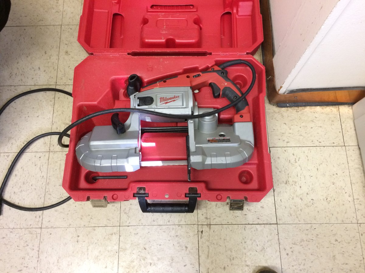
For cutting, I have this nice portable band saw and table.  I bought this particular tool several years ago and it has saved me hours if not days of work at various sites.  I have used it to cut not just coaxial line and cables, but uni strut, threaded rod, copper pipe, coolant line, conduit, wire trays, etc.  If you are doing any type of metalwork that involves cutting, this tool is highly recommended.

Milwaukee 6230N Band Saw with cutting table

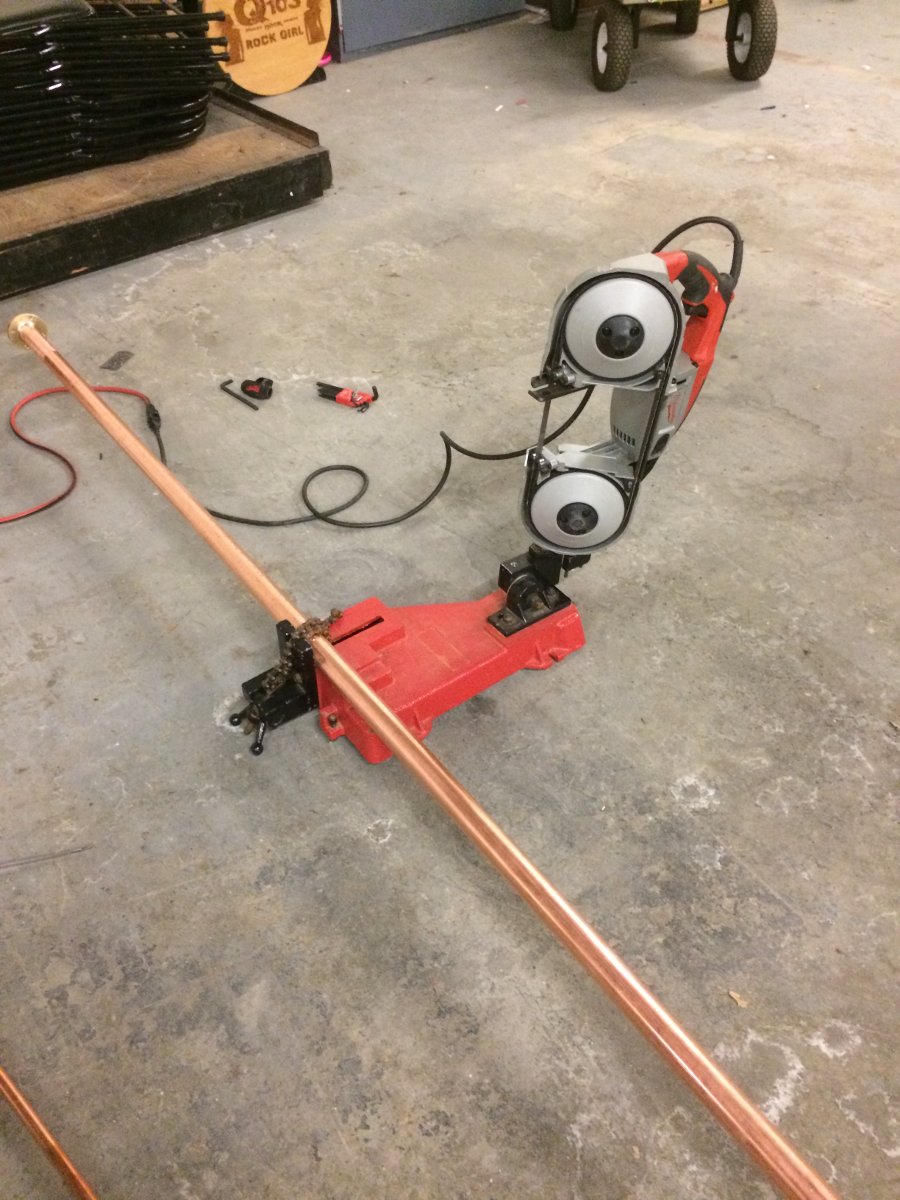
There are now Lion battery types of bandsaws which are certainly more portable than this. Still, the table with the chain clamp makes work much easier and the cuts are straight (perpendicular), which in turn makes the entire installation easier.

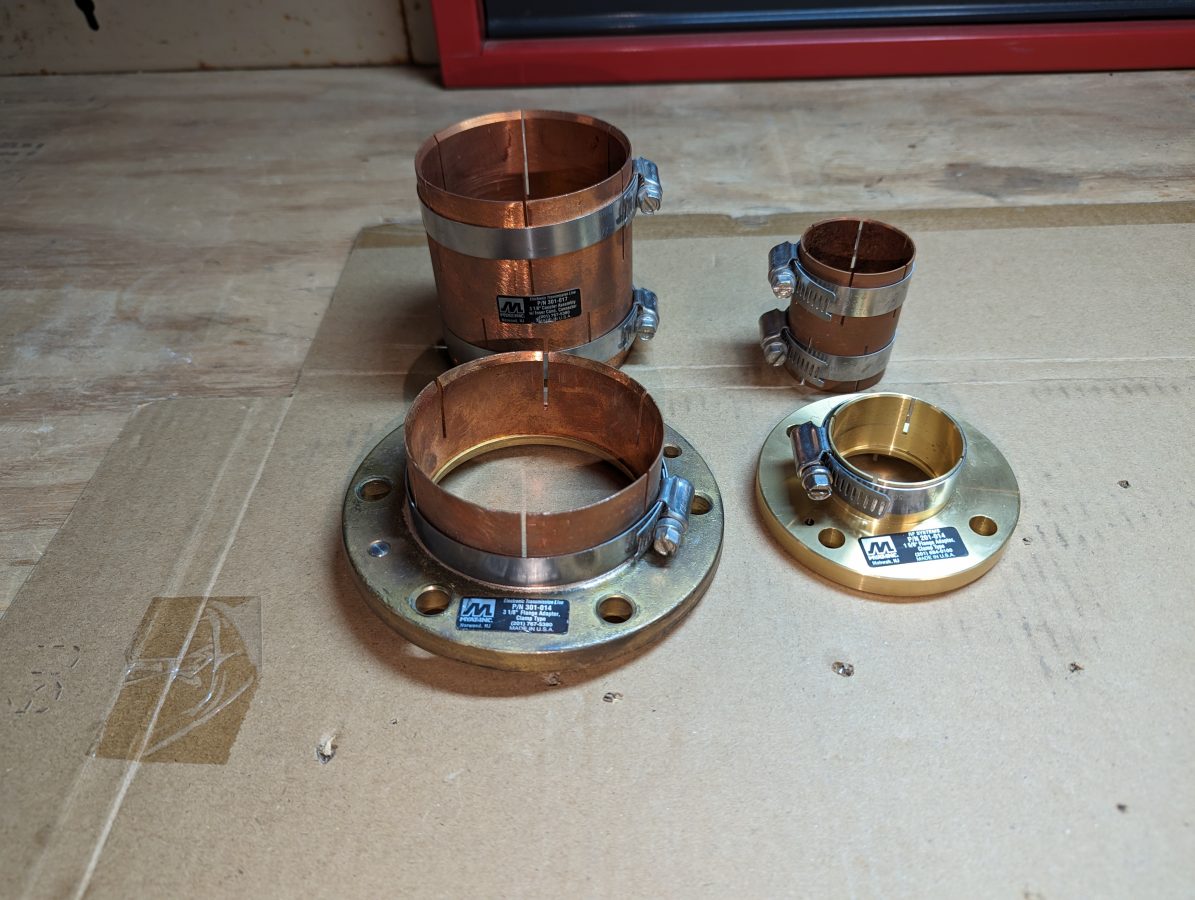
The next point is how long to cut the line pieces and still accommodate field flanges and inter-bay line anchors (AKA bullets). 

Inner bay line anchor, aka “bullet” 3 1/8 inch, 1 5/8 inch, and 7/8 inch respectively

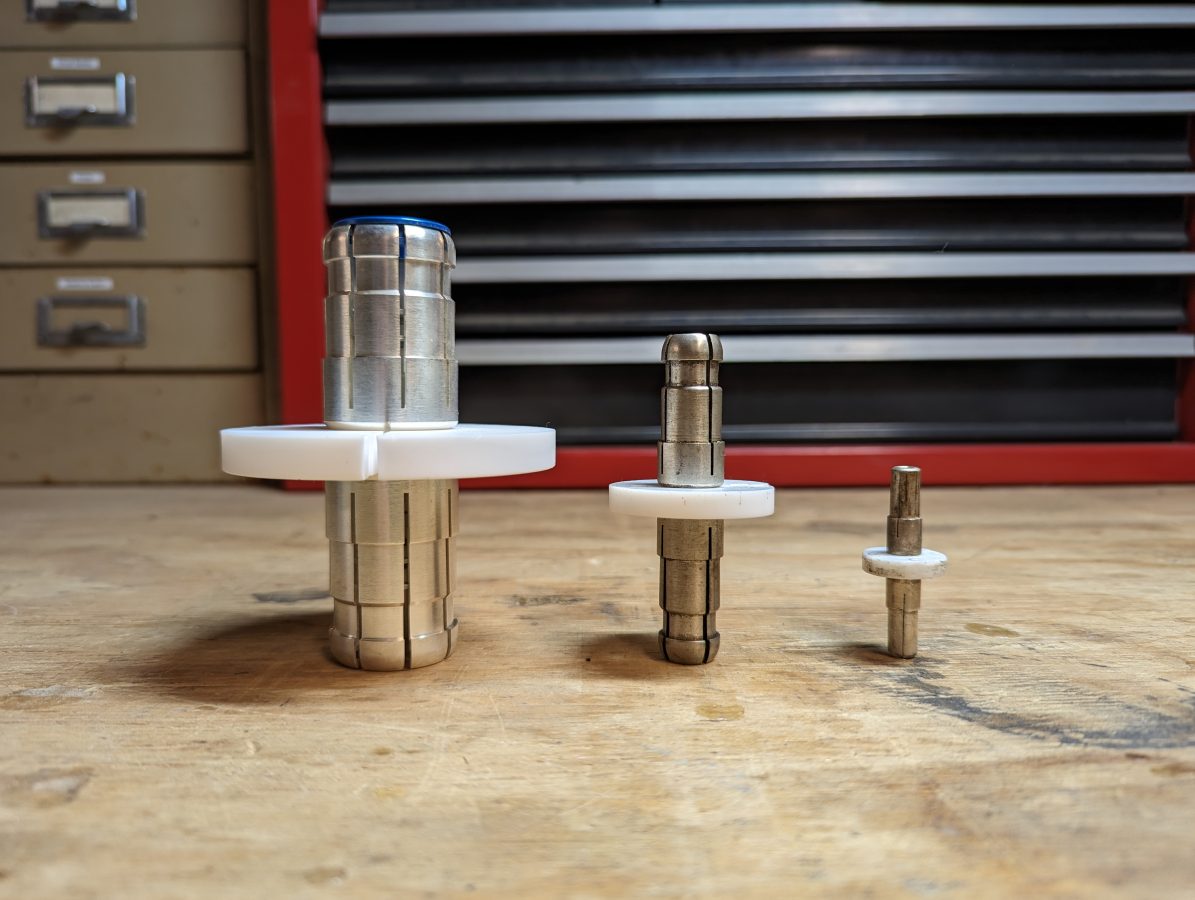
The inner conductor is always going to be shorter than the outer conductor by some amount.   Below is a chart with the dimensions of various types of rigid coaxial cables.

Length cut chart for various sizes of rigid coaxial cables

When working with 1 5/8 inch rigid coax, for example, the outer conductor is cut 0.187 inches (0.47 cm) shorter than the measured distance to accommodate the field flange. The inner conductor is cut 0.438 inches (1.11 cm) shorter (dimension “D” in the above diagram) than the outer conductor to accommodate the inter-bay anchors. These are per side, so the inner conductor will actually be 0.876 inches (2.22 cm) shorter than the outer conductor.  Incidentally, I find it is easier to work in metric as it is much easier to measure out 2.22 CM than to try and convert 0.876 inches to some fraction commonly found on a tape measure.  For this reason, I always have a metric ruler in my tool kit.

If you do not have a handy chart, you can estimate the inner conductor length by measuring the inner bay anchor from the insulator to the first shoulder. Then multiply by two.

Measuring inner bay line anchor

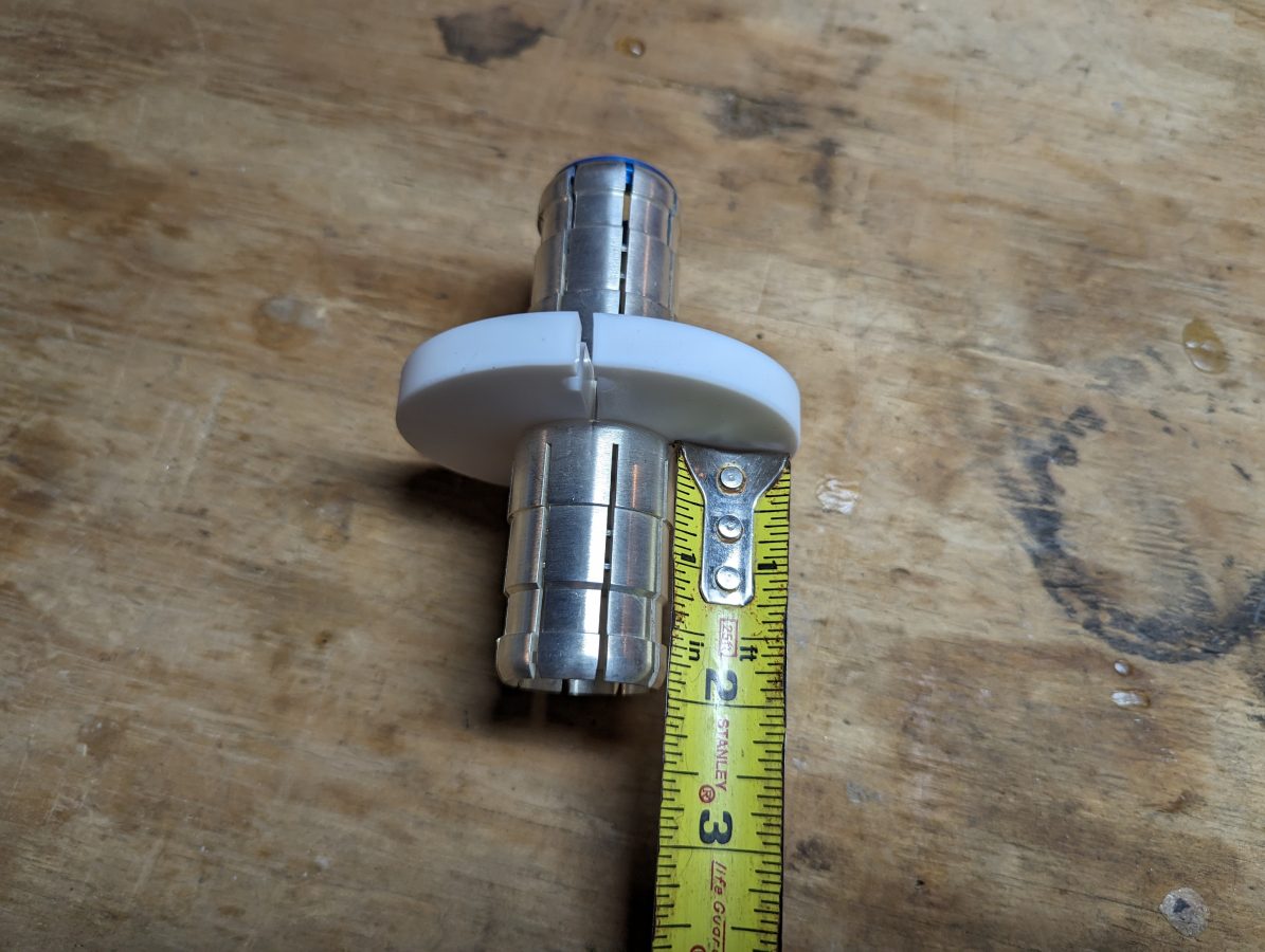
In this case, the measurement from insulator to shoulder is 11/16th of an inch (17.5 mm). If Clamp On Flange adaptors (AKA field flanges) are being used, don’t forget to account for the small lip (usually less than 1/16th of an inch) around the inside of the flange where the outer conductor is seated. If you are using unflanged couplings instead of field flanges, then you can disregard this.

Clamp on Flange adaptors in the front, flangeless couplers in the back
Altronic air cooled 20 KW test load
1 5/8 inch rigid coax run to Altronic air-cooled 20 KW test load
1 5/8 inch rigid coax and 4 port coax switch mounted in top of Middle Atlantic Rack
1 5/8 inch rigid coax and 4 port coax switch mounted on top of Middle Atlantic Rack

The next step is de-burring.  This is really critical at high power levels.  I use a copper de-burring tool commonly used by plumbers and electricians.

De-burring tool, can be found in the plumbing isle of most big box hardware stors

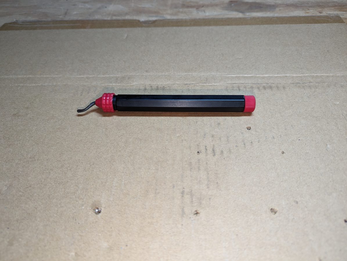
One could also use a round or rat tail file to de-bur.  The grace of clamp-on field flanges is they have some small amount of play in how far onto the rigid line they are clamped.  This can be used to offset any small measurement errors and make the installation look good.

Radio Guide; The Magazine

As some of you may have noticed, recently I have been writing some articles for Radio Guide. There are several good reasons for this, but the most important one is education. I believe that terrestrial radio will be around for a few more years. As others have noted, there are fewer and fewer broadcast engineers. Those that understand high-power RF and all its intricacies are fewer still. It is important that a cadre of knowledgeable broadcast engineers carry on.

The internet is a great thing. However, it depends on cables of some type to exist. As we know, cables can be damaged. In addition to cables, there are routers, core switches, servers, and so on. All of that equipment can fail for various reasons. People have been working hard to improve the resiliency of the internet. That is a good cause, to be sure. However small it may be, there is still a chance that the internet can fail. Worse still, this can happen during some type of natural disaster or other emergency. Thus, during such an emergency, Radio can and will function as a vital information source provided that the station is on the air and has a program feed. That is also a good reason to keep the current RF STL paths in place as much as possible.

The Radio Guide articles are a great way to pass along some of that hard-earned experience to others. I also want to put supplemental information here for those interested to download. Things like charts, forms, pictures, videos, etc.

What I am planning on is to list the articles here, then put links to any supplemental information provided below that subheading.

Designing an ATU

Most ordinary field engineers will not need to design an ATU in the course of their normal duties. However, knowing the theory behind it can be very helpful when troubleshooting problems.  Also, fewer and fewer people understand RF these days, especially when it comes to AM.  Knowing a little bit can be an advantage.

We were working on an AM tower recently when several discrepancies were noted in the ATU:

WFAS ATU, 1230 KHz
WFAS ATU, 1230 KHz, 1 KW, N-DA

This was connected to a 202° tower. There were several complaints about seasonal shifts and narrow bandwidth. The VSWR meter would deflect slightly on high-frequency audio peaks, always a bad sign.  A little bit of backstory is in order.  WFAS signed on in 1930 using a four-legged self-supporting tower.  This tower was used until about 1986, when it was replaced with a series excited, guyed tower.  The ATU in use was initially designed for the replacement tower, which likely had a good bit of capacitive reactance.  I am speculating on that, as I cannot find the original paperwork for the replacement tower project.  At some point, somebody decided to ground the tower and put a skirt on it, likely to facilitate tower leasing.  The skirt was installed, but the ATU was never properly reconfigured for the high inductive reactance from the skirted tower.  The truth is, the Collins 820-D2 or Gates BC-1G tube-type transmitters probably didn’t care.  They were probably like; bad load, meh, WHATEVER!  Although the audio quality likely suffered.  That all changed when Broadcast Electronics AM1A was installed.  To fix the bad load problem, a BE 1 KW tuning unit was installed next to the transmitter.

Technically, there are several problems with the above circuit, starting with the capacitor on the wrong side of the base current meter.  This capacitor was installed outside of the ATU between the tower and ATU output.  Was the base current meter really measuring the base current?  I don’t know, maybe? The shunt leg was lifted but both of the inductors of the former T network were left in the circuit.

We reconnected the shunt leg and moved the capacitor inside the ATU and to the correct side of the base current meter.   After several hours of tuning and fooling around with it, the ATU is still narrow-banded, although now at least the input is 50Ω j0. I believe the current design has too much series inductance to be effective.

Thus, a redesign is needed.  I think, because of the inductive reactance of a skirted tower, a phase advance T network will lead to best bandwidth performance.  The basic design for a +90-degree phase advance looks like this:

WFAS -90 lagging ATU
WFAS +90 phase advance ATU, 1230 KHz, 1 KW, N-DA

To calculate the component values for the ATU, some basic arithmetic is required.  The impedance value for each leg in a +/- 90 degree T network can be calculated with the following formula:

Z = √(inputZ × outputZ)

Where Z = impedance per leg
Input Z = the ATU input impedance, 50Ω
Output Z = the antenna resistance, 58Ω

Thus:  Z =√ (50Ω × 58Ω)

Z = 53.85Ω

Formula for Capacitance: C = 1/(2Π × freq × XC)

Thus for the input leg: C = 1/(6.28 × 1.23MHz × 53.85Ω)

C (input)  = 0.0024 μF

Formula for Inductance:  L = XL/(2Π × freq)

Thus for the shut leg: L = 53.85Ω /(6.28 × 1.23 MHz)

L (shunt) = 6.97 μH

For the output leg, we must also consider the inductive reactance from the tower which needs to be cancelled out with capacitance.  Thus, the output capacitor needs to have a value of 53.85Ω + 580Ω = 633.85Ω

Thus for the output leg: C = 1/(6.28 × 1.23MHz × 633.85Ω)

C (output)  = 0.000204 μF

The amazing thing is, all of these components are available in the current ATU, they just needed to be rearranged.  The exception is the vacuum variable capacitor, which I salvaged from an MW-5 transmitter many years ago.  I donated that to the project, as I am tired of looking at it in my basement.  The reason for the vacuum variable capacitor will become evident in a moment.  The input capacitor will be slightly over value, which will require the inductor to tune out the excess capacitance.  A good design rule is to use minimum inductance to adjust the value of a fixed capacitor, thus the capacitor should be not more than 130% of the required value.

About the Vacuum variable output capacitor; in the existing ATU had a 0.0002 μF capacitor already.  With a +90° phase shift, this capacitor is likely adequate for the job.  The vacuum variable may be pressed into service if something other than a +90° phase shift is needed for optimum bandwidth.  That will be the topic of my next post.

Final consideration is the current and voltage ratings of the component.  As this is a re-build using existing components, chances are that they already meet the requirements.  On a new build or for replacing parts, one must consider the carrier power and modulation as well as any asymmetrical component to the modulation index.  For current and voltage each, the value is multiplied by 1.25 and then added to itself.  For a 1,000 watt carrier the input voltage on a 50 ohm line will be approximately 525 volts at 10 amps with 125% modulation.  A good design calls for a safety factor of two, thus the minimum rating for component in this ATU should be 1050 volts at 20 amps, rounded up to the next standard rating.   The capacitor on the output leg should be extra beefy to handle any lightning related surges.

The current rating for a capacitor is usually specified at 1 MHz.  To convert to the carrier frequency, the rating needs to be adjusted using the following equation:

IO = IR√ FO

Where:
IO: current rating on the operating frequency
IR: current rating at 1 MHz (given)
FO: operating frequency in MHz

The vacuum variable output capacitor is rated for 15,000 volts, 42 amps.  Adjusted for frequency, that changes to 46 amps.  The calculated base current is 4.18 amps carrier, 9.41 amps peak modulation.  Thus, the capacitor on hand is more than adequate for the application.

The Smith Chart

I have been fooling around with Smith Charts lately. They look complicated, but are really pretty easy to understand and use, once you get around all those lines and numbers and stuff. Smith charts offer a great way to visualize what is going on with a particular antenna or transmission line. They can be very useful for AM antenna broadbanding.

Smith chart
Smith chart

.pdf version available here: smith-chart.

The first thing to understand about a Smith chart is normalization. Impedance and reactance are expressed as ratios of value units like VSWR. A ratio of 1:1 is a perfect match. In the center of the Smith chart is point 1, which expresses a perfect match. To normalize, the load resistance and reactance are divided by the input resistance. Thus, if the input resistance is 50 ohms and the load impedance is 50 ohms j0, then the normalized Smith chart point would be 50/50 or 1. If the load impedance is 85 ohms and the reactance is +j60, then the normalized Smith chart point would be .58 1.7,1.2.

More basic Smitch chart usage information in this video:

I touched on the black art of AM antenna broadbanding before. It is a complex topic, especially where directional antenna systems are concerned, as there are several potential bottlenecks in a directional array. To explain this simply, I will use an example of a single-tower non-directional antenna.

Below is a chart of base impedance from a single tower AM antenna on 1430 KHz.  The tower is skirted, 125.6 degrees tall.  An AM tower that is expressed in electrical degrees is denoting wavelength.  A 1/4-wave tower (typical for AM) is 90 degrees tall. A 1/2 wave tower is 180 degrees tall.  Thus this tower is slightly taller than 1/4 wavelength.

Frequnecy(khz)ReactanceReactance (normalized)ResistanceResistance(normalized)
1390-j 139-2.784058.1
1395-j 143-2.864008.0
1400-j 147-2.943507.0
1405-j 146-2.923106.2
1410-j 142-2.842705.4
1415-j 132-2.642364.72
1420-j 125-2.502104.2
1425-j 118-2.361903.8
1430-j 112-2.241703.4
1435-j 106-2.121553.1
1440-j 100-2.001382.76
1445-j 93-1.861252.5
1450-j 86-1.721142.28
1455-j 79-1.581042.08
1460-j 75-1.50951.9
1465-j 70-1.4921.84
1470-j 65-1.3851.7

The base impedance is not too far out of line from what is expected for a tower this tall.  Plotted on a Smith Chart:

1430 base impedance plotted on a Smith chart

One of the first principles behind broadbanding an AM antenna is to distribute the sideband energy evenly and have a symmetrical VSWR.  The antenna tuning unit will match the line impedance to the load impedance and cancel out the reactance.  Having the proper phase advance or phase retard rotation will distribute the sideband energy symmetrically about the carrier.   To determine phase rotation, the cusp of the plotted graph is rotated to face either the 3 o’clock or 9 o’clock position (0° or 180°).  The cusp is where the direction of the line changes, which in this case is the carrier frequency, 1430 KHz.  The above example, the line is fairly shallow, which is typical of a skirted tower.  Thus, the best phase rotation to start with is +79°.  This will likely be close but will need to be tweaked a bit to find the optimum bandwidth.  After looking at the plotted Smith chart, my first inclination would be to reduce the rotation, more tower +75° as a first step in tweaking.

When working with AM systems, the bandwidth of the entire system needs to be examined.  That means that final bandwidth observations will need to be made at the transmitter output terminal or in some cases, the input to the matching network.  It varies on system design, but things like switches, contactors, mating connectors, ATU enclosures, etc can also add VSWR and asymmetry.  Broadbanding even a simple one-tower AM antenna can require quite a bit of time and some trial and error.

I will touch on ATU design in the next post.