A story about skirted AM towers and Cellular carriers.
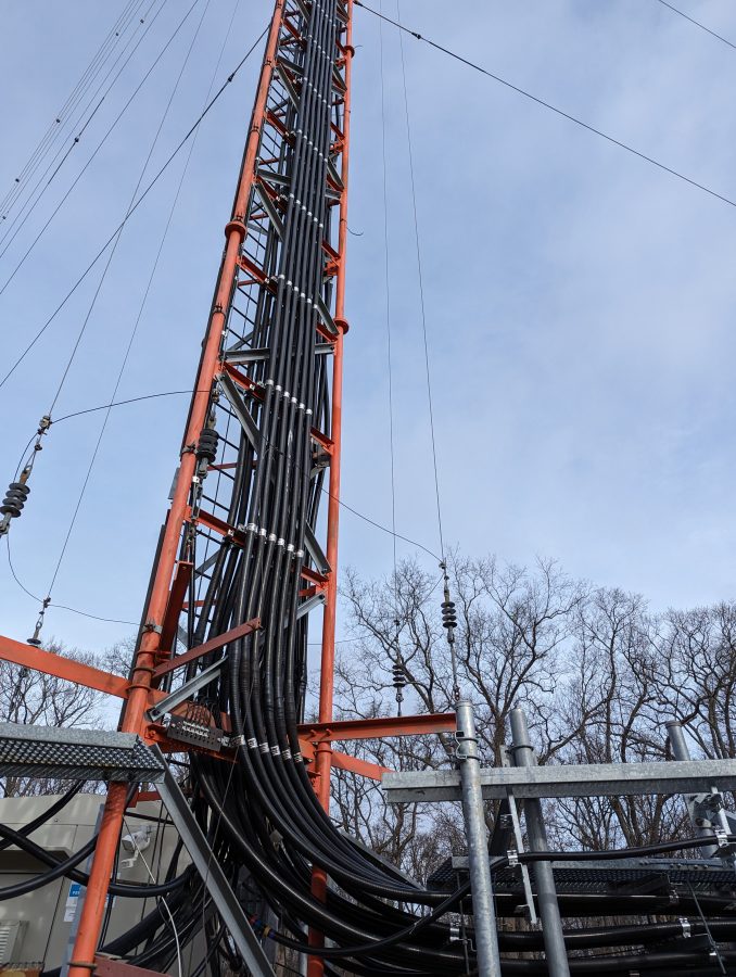
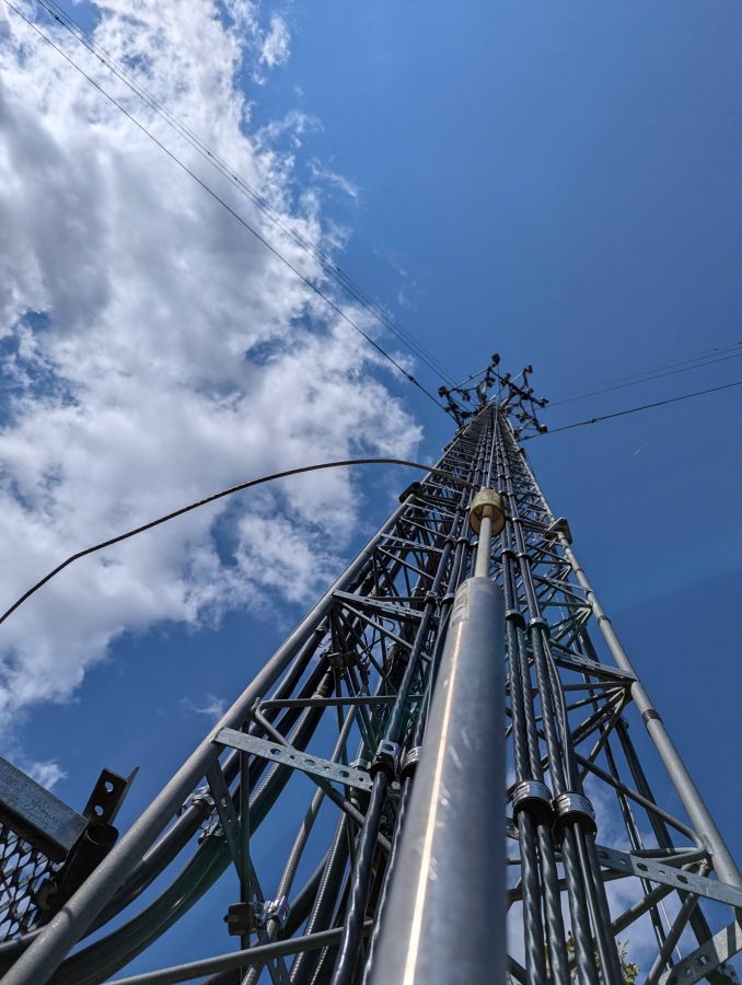
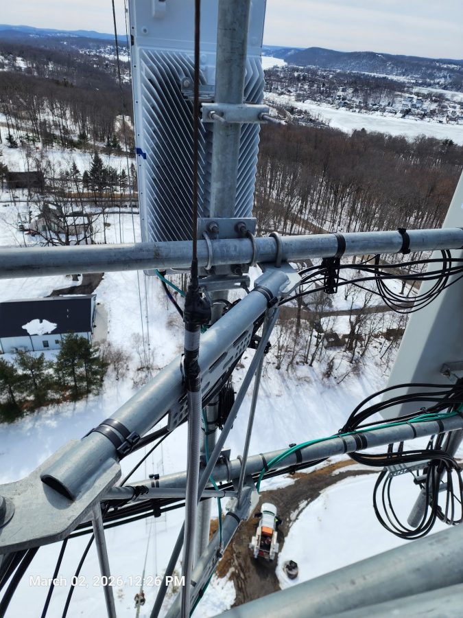
Skirted AM tower with cellular equipment
We take care of a few sites that have skirted AM towers with Cellular equipment installed. For the first few years, all was well. The cell carriers put up their equipment under supervision and we made sure that the AM station’s antenna still was working when the were finished. At some point, things changed.
Stiff arm hitting skirt wire
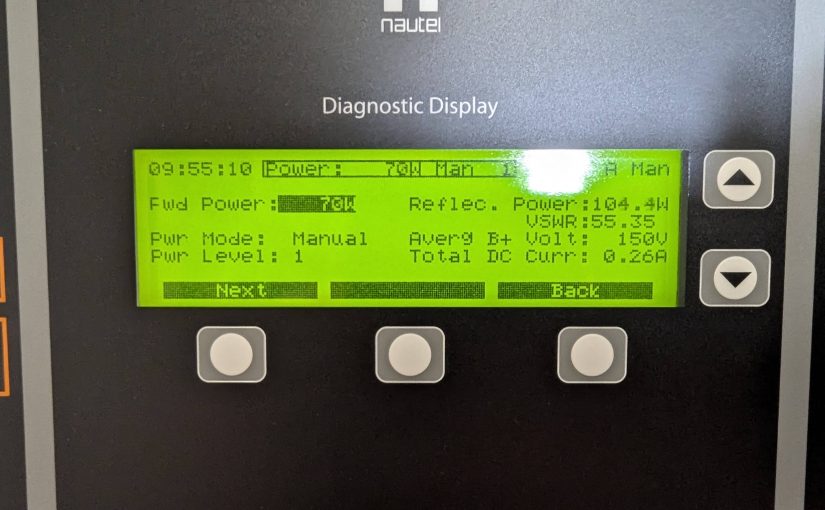
It is a little bit hard to see because the camera is focused on the foreground and not the background, but the stiff arm from the cell carrier sector is shorting the skirt wire to the tower.
More often then not these days, tower crews show up unannounced and start working on the tower. I had a call from a client their station being off the air only to arrive on site and find a crew on the tower with the AM skirt grounded by a set of battery jumper cables. The ground crew said they kept getting shocked by the wire so they grounded it.
In other cases, they show up, do the work and leave before anybody notices. Then, at some point somebody checks the AM transmitter readings and sees a problem.
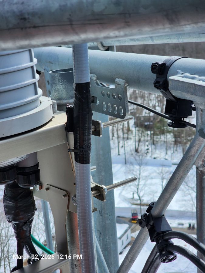
AM skirt wire, shorting against mounting bracket
In another situation, the tower crew came and installed new equipment. They installed an insulating sleeve around the skirt wire (while the transmitter was on) but did not secure it well enough. The eventually, sleeve slipped down the wire and it shorted. No one, not even the tower owner, knew about the tower crew being on the tower.
AM skirt wire insulating sleeve
Same tower, the sleeve on this wire rotated around so that the opening was facing the stiff arm causing a large charred, melted plastic area.
These were repaired with some left over coax-seal and electrical tape. After this, I was able to retune the ATU using my network analyzer.
The only solution, it seems, is to put up more cameras with motion detection notification so when somebody shows up unannounced the station will at least know about it.
This has nothing to do with broadcasting. It does, however, have a good deal of geeky goodness.
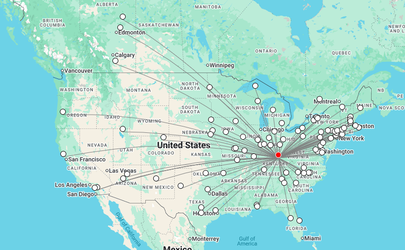
I have started a new project, getting on the air on the 630 meter Amateur band. For those who do not know, 630 meters is from 472–479 kHz which is below the AM (or Standard) broadcast band. It was formerly part of the Maritime Mobile allocation. For US Amateurs, these frequencies were added in 2017 so it is a relatively new experience.
There is no commercially available equipment for this band, so it depends on the potential operator to make his or her own equipment which is where the fun begins.
To start, I thought I’d repurpose a WSPR beacon to 630 meters to do some antenna experimentation. Like all transmitters, the output of this unit needs to be filtered to reduce or eliminate out of band emissions. The Amateur radio service falls under Part 97, which has somewhat different requirements than Part 73 or 74.
47CFR 97.307(d) states:
For transmitters installed after January 1, 2003, the mean power of any spurious emission from a station transmitter or external RF power amplifier transmitting on a frequency below 30 MHz must be at least 43 dB below the mean power of the fundamental emission.
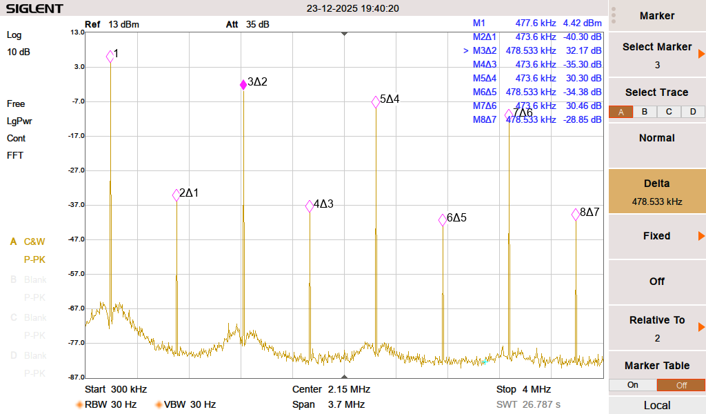
That is a fairly low bar. I am going to shoot for something better. WSPR beacons center around 475.6 kHz. The harmonics are at 951, 1428, 1902, 2378, 2853, 3329, 3804, 4280 and 4756 KHz. The first two are in the AM broadcast band. A quick look at the Zachtek WSPR beacon show these harmonics:
unfiltered ZackTek WSPR Desktop transmitter, 630 meter band
Definitely does not meet the out of band emissions standard set forth in FCC 97.307. Typical of solid state amplifiers, the odd harmonics are greater than the even.
I used a filter design program called Elsie to design suitable filters for 630 Meters. There are two types of filters that can attenuate the harmonics; low pass and band pass. A low pass filter passes all emissions below the cutoff.
630 Meter low pass filter
That is fine, however, it does not eliminate the possibility of interference and inter- modulation from frequencies below the band. Both types of filters are also good for receivers in the presence of AM broadcast band towers, which can desensitize receiver front ends when located nearby.
A band pass filter cuts off frequencies above and below the pass band.
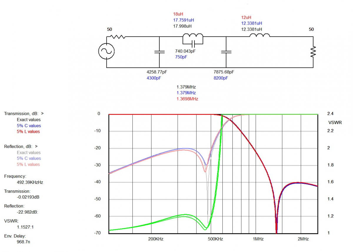
630 Meter band pass filter
This is a nodal inductor-coupled band pass filter. I like this design because it has deep shoulders and has better performance with the harmonics in the AM broadcast band.
Prototype low pass filter:
630 Meter Low Pass Filter
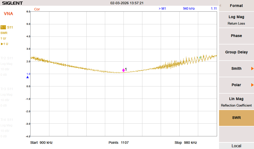
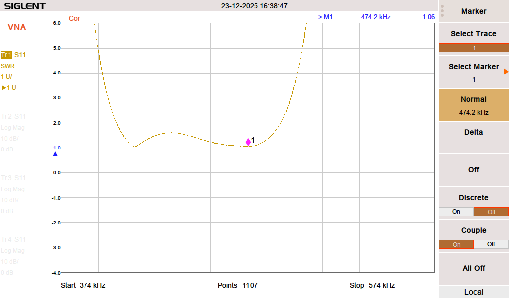
Quick prototype board. Capacitors are Cornell Dubilier silver mica dipped, the inductors are wound on T130-3 material. The SWR and return loss:
Smith chart:
The Smith chart shows that it is slightly inductive on the desired frequency. The way to mitigate is to either add some capacitance (not easy) or reduce the inductance (somewhat easier). I tried tuning it by changing the spacing on the windings of L1 and L2. There was no change.
Low pass filter response:
The second harmonic on 951 KHz is -58.37 dBc. Harmonics 3 – 7 are 40 dB below the fundamental. This is adequate but the band pass filter below is better.
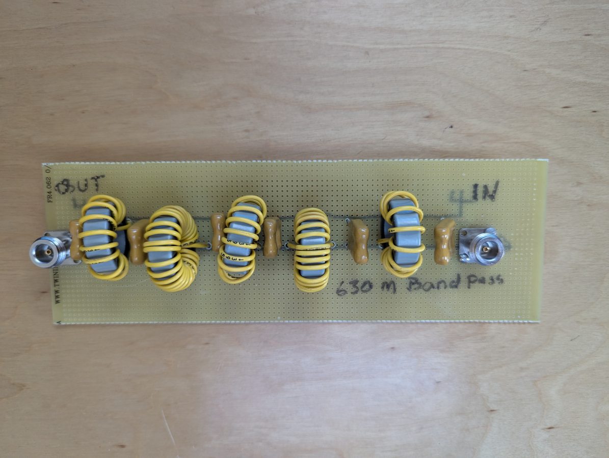
Prototype band pass filter:
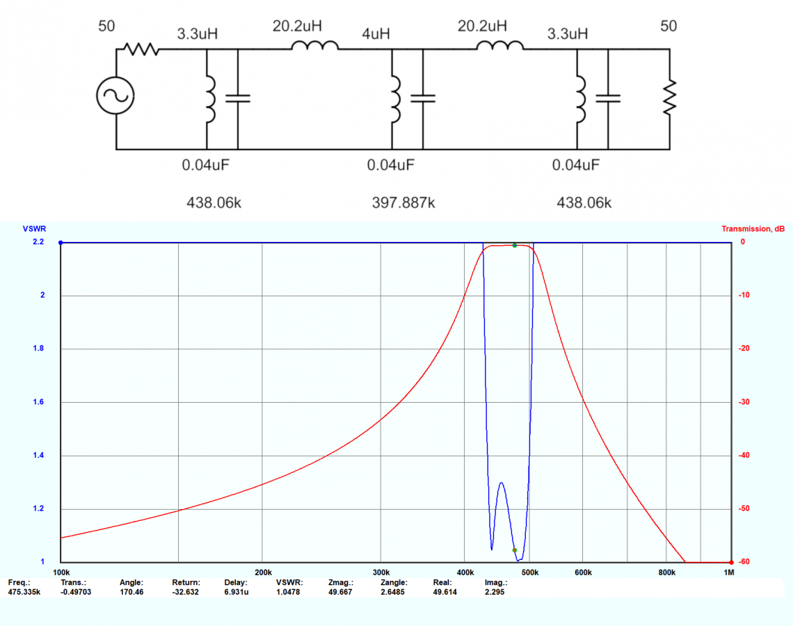
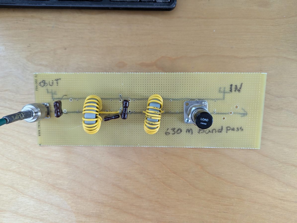
630 Meter band pass filter prototype
The above filter is a little rough, but it was a good test of the filter program’s design parameters. The capacitors are Cornell Dubilier 0.02 uF 500V. The inductors are wound on T130-3 iron powder toroid cores. The results are good:
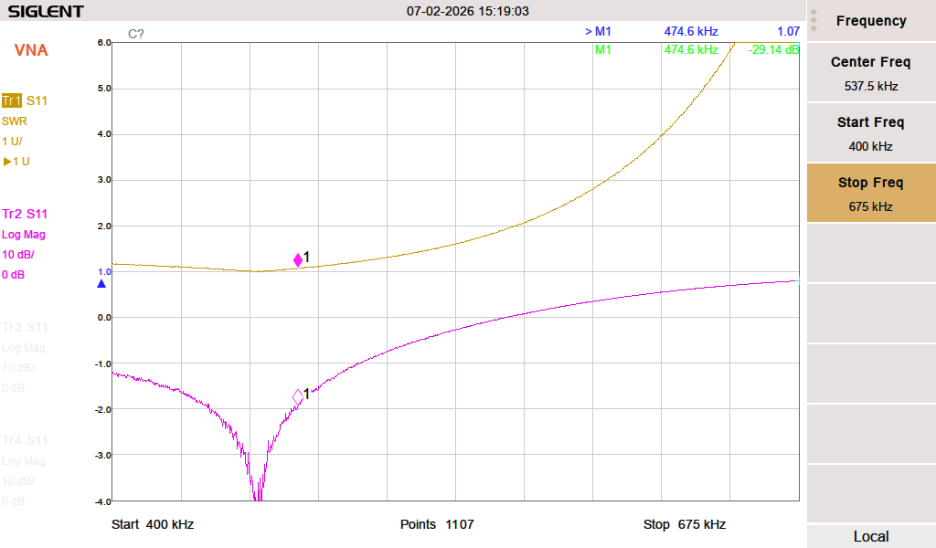
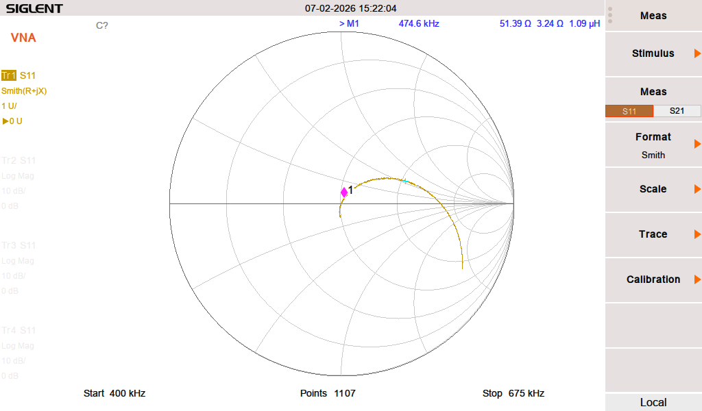
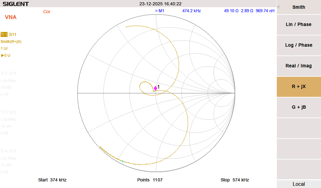
630 Meter band pass smith chart
By adjusting the spacing of the windings on L3 (center of the board), I can tune the VSWR and Return loss for best values.
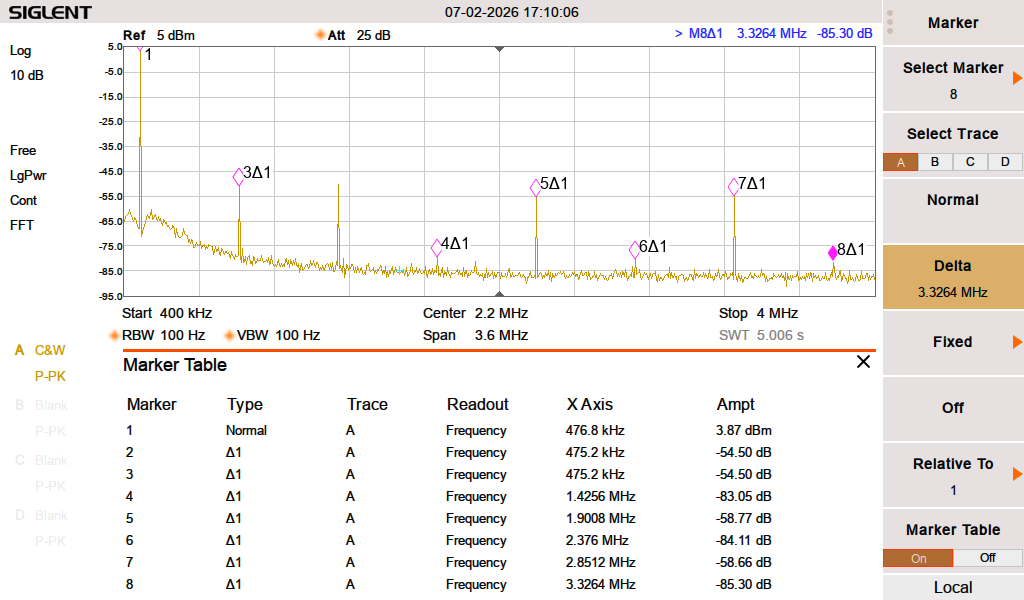
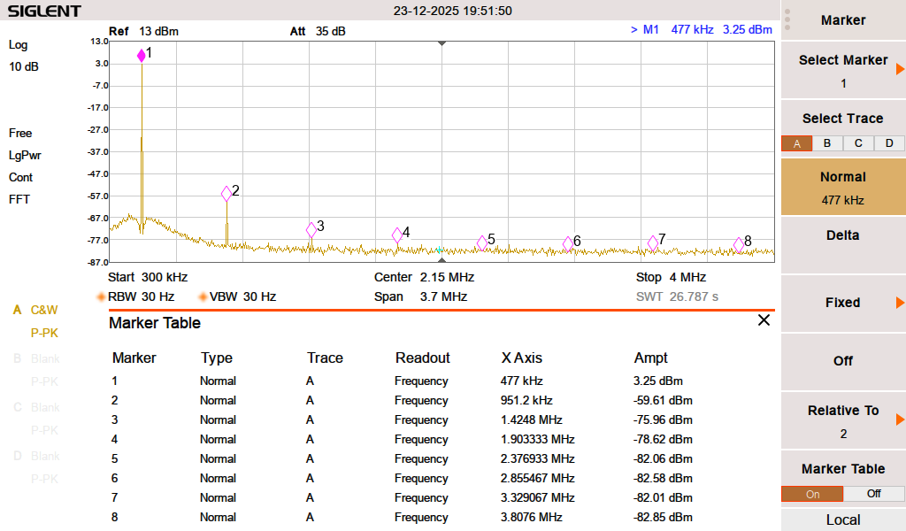
The same ZachTek WSPR transmitter noted above, running through the prototype filter:
ZachTek 630 Meter band pass filter response
The second harmonic on 951 KHz is -62.86 dBc. The rest of the harmonics are less than that.
Of the two, the band pass filter has better performance characteristics. The return loss/SWR is lower and can be tuned by adjusting the spacing of the toroid windings on L3.
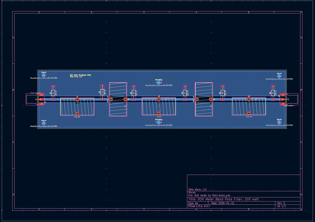
I decided to take the next step and make a PCB. I have KiCad on my Linux machine, which works well. Sometimes some of the foot prints need to be edited so the dimensions are correct, but that is easy.
KiCad design 630 meter band pass filter
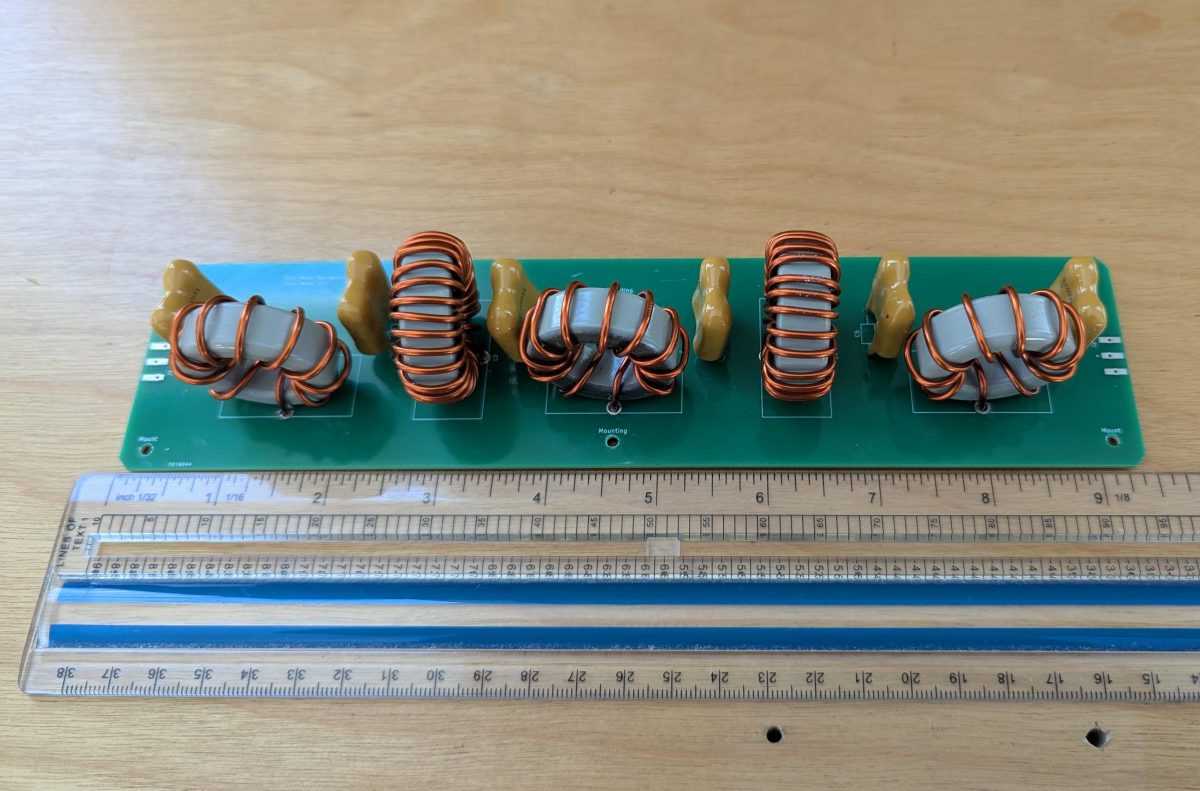
What I like about this board design is that it will work on any amateur band below 7 MHz with different component values. I had five boards fabricated and built one of them out. The T130-3 toroids are wound with 14 AWG magnet wire. The capacitors are same used in the prototype, 0.02 uF, 500V mica dipped.
Cleaned up band pass filter board
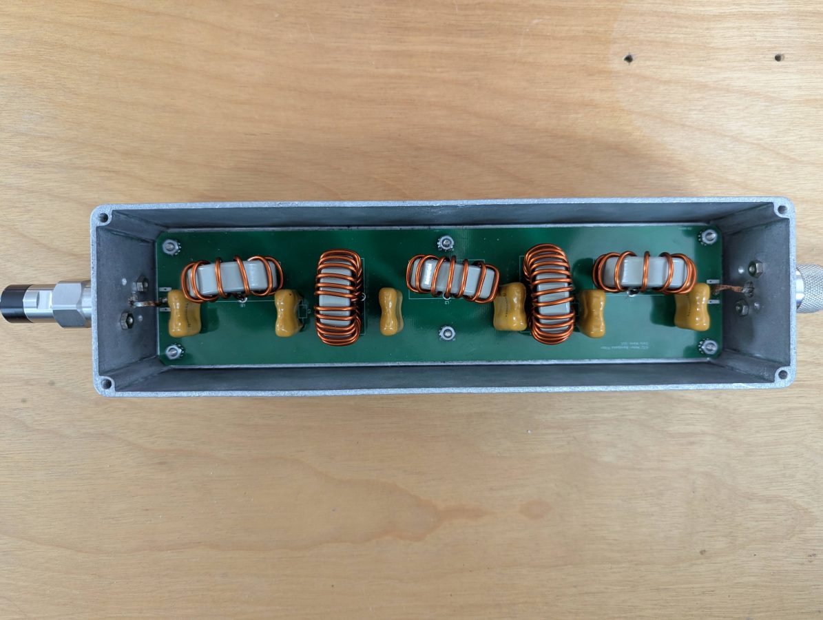
Board mounted in aluminum enclosure:
Band pass filter mounted in diecast aluminum enclosure
This build has similar measurements to the prototype board above. Based on what I found while making this, I made a few tweaks to the circuit board in KiCad. I would consider selling these, if there is enough interest.
NOAA All Hazards Radio has been around since 1960. I have a Midland Weather Radio receiver in my house because we live in a rural area. We certainly do have weather events; Severe Thunderstorms being the most common. We have also had Tornados, Floods, Hurricanes, Winter Storms and Blizzards. It is useful to have, especially when the cell phone and/or public network go down.
That system operates on the same frequencies and manner as the NOAA All Hazards Radio system.
It appears that the Canadian government is discontinuing service as of March 16, 2026 and replacing it with an app. That seems short sighted to me; I don’t know how many users of Weather Radio Canada there are, but I’d bet there are quite a few. It also assumes that everyone in Canada has a smart phone. Given the economy and the expense of a new iPhone (or Android), I think this is far from the case.
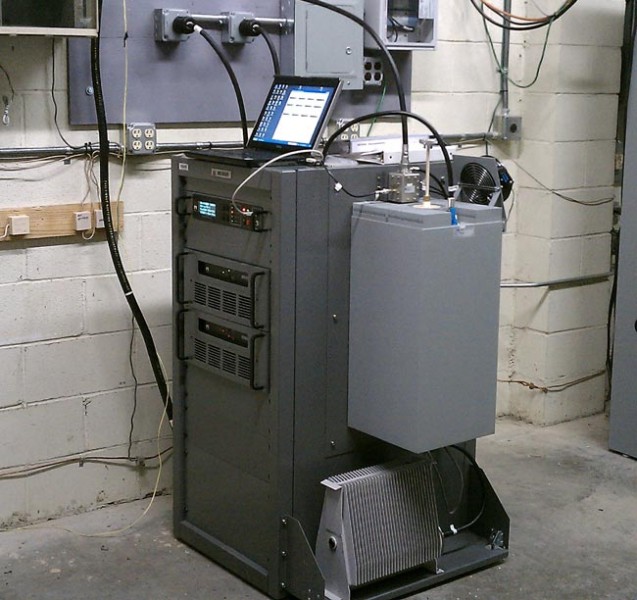
Nautel NG1000 NOAA transmitter
I did get thinking about what would happen here if the NOAA system went away. Could the Emergency Alert System still get reliable local alerts out over the air? I know that most of the radio and TV stations in this area still monitor the NOAA frequencies as a third source for local activations. Over the years, EAS activation for things like Tornado Warnings has saved quite a few lives, especially out in the mid west.
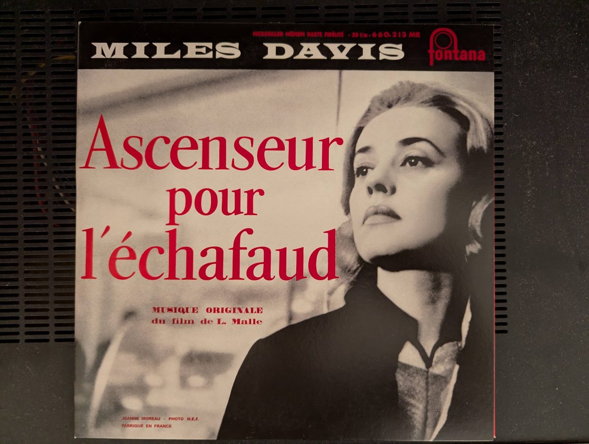
I am seeing more and more people getting into (or back into) vinyl recordings. This is somewhat heartening. My personal feeling is that good analog recordings offer a great way to enjoy music, particularly older music. The other nice thing; when I am holding a physical disk, it is mine. I bought it, I own it. No one can track it or delete it from my device.
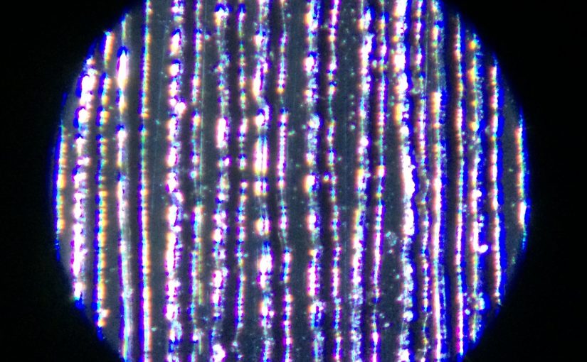
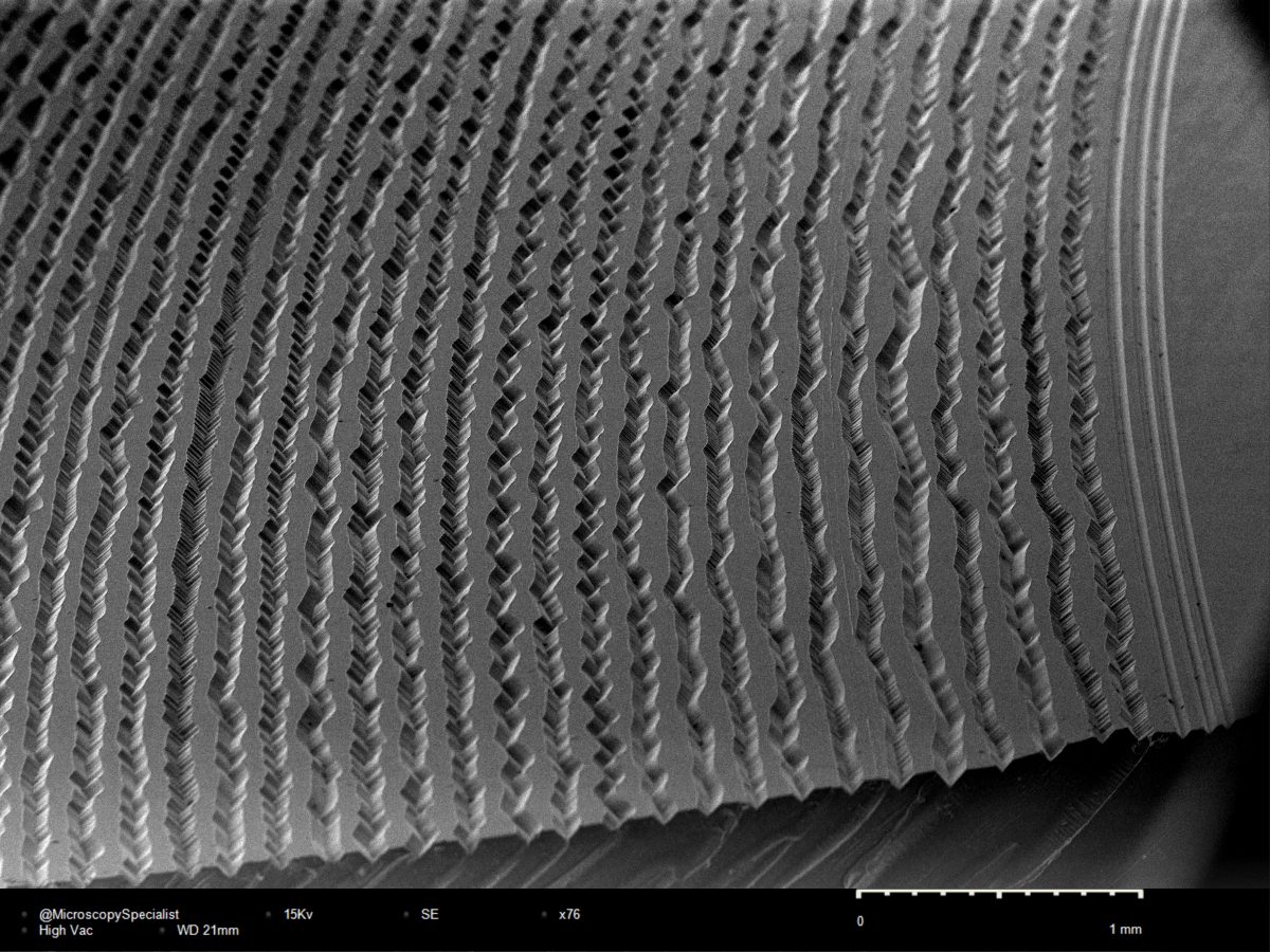
Grooves in a vinyl disk seen through an electron microsope, courtesy of Eric Muzipov @microscopyspecialist
Vinyl is actually Polyvinyl Chloride or PVC. Columbia records switched from Shellac record disks to PVC around 1947. According the the RIAA, vinyl sales peaked in the US around 1973. It is possible to find new vinyl in a few places like Target, Walmart and Barnes & Noble. There is a large market for used vinyl recordings in local record stores like Dark Side Records.
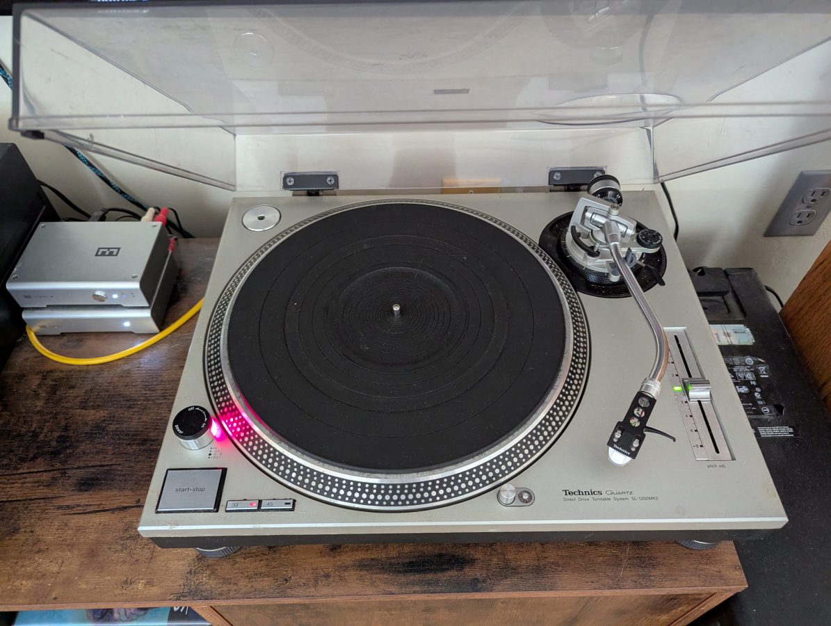
Technics SL-1200 Mk II turntable
Many years ago, I retrieved this Technics SL-1200 Mk II turntable from the trash heap. This particular turntable had been through the flood after Hurricane Irene (2011). It spent more than 48 hours completely submerged in some pretty dank water. Following that, it went into the barn for many years without being looked at.
At some point in the last few years, I decided that I wanted a turn table for my Hi-Fi system. I retrieved the Technics unit from the barn and began the rehab. Fortunately, both the service manual and user manual are easy to find on line.
I disassembled the entire unit and inspected all of the parts. As it turned out, it was fresh water and the damage did not look too bad. There is some pitting on the under side of the platter and some general corrosion on the strobe dots. It took a while and a good deal of patience and elbow grease to clean everything off. The electronics in this turn table are only for control of the direct drive motor. Audio passes through to the outboard pre-amp. There is one 450 uF 50 VDC capacitor in the power supply which looked good, so I left it alone.
I put it all back together, but realized quickly that it needed to be set up correctly. There are many videos on Youtube that show how to align this particular model turntable. A complete alignment is important because the stylus must meet the grove at the correct depth and angle in order for the playback to be accurate.
The mechanical setup consists of five main things;
The turn table must be completely level front to back and especially center post to stylus (the track of the tone arm)
The height of the tone arm (stylus angle in the groove)
The vertical tracking weight (proper frequency response, stylus and record wear)
The anti-skating (proper pressure on both sides of the record groove, correct amplitude)
Alignment of the cartridge in the cartridge head (stylus angle in the groove, proper left/right phasing, stereo separation and image)
These items are very easy to deal with on the SL-1200. It has feet that can be adjusted to level the unit. The leveling of the tone arm track is especially important to get right.
The height of the tone arm is set with the base arm ring. Some turntables do not have this adjustment, particularly consumer grade units. The tone arm should be level when the stylus is on the record.
The tracking weight is set by the tone arm balance weight. First, the tone arm is balanced so that it floats (in other words zero weight). The tracking weight depends on the cartridge and stylus being used. In this case, the cartridge is an Audio Technica AT-OC9XEN Moving Coil cartridge with an elliptical stylus. The tracking weight for that cartridge is 1.8 to 2.2 grams. I set mine to 2.0 grams.
Anti-skating is generally set for the same value as the tracking weight. However, this is sometimes too coarse. A test record with a blank band on it can help get this exact. It does not make a huge difference, but it is nice to confirm this anyway.
The alignment of the cartridge in the head shell is important, especially with an elliptical stylus. This is done using a Cartridge Alignment Protractor which can be downloaded for free from the vinylengine.com website
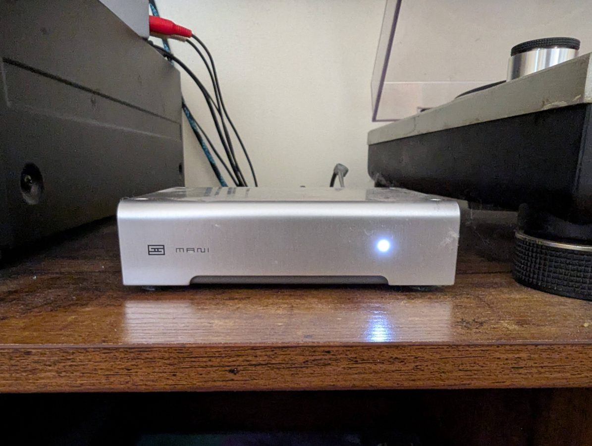
Schiit Audio, Mani phono pre-amp
I purchased this piece of Schiit a few years ago to use with my vacuum tube amplifier. I have since switched to a Kenwood VR309 for my main listening setup. While the phone preamp in my Kenwood stereo is pretty good, I think this preamp sounds better, especially with the moving coil stylus.
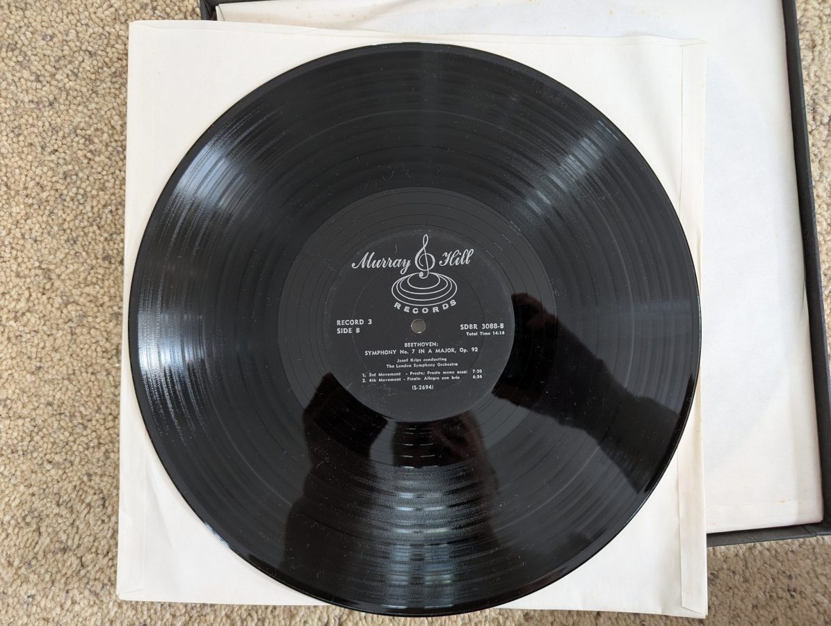
Circa 1960 Beethoven Symphony No. 7 in A Major. Murray Hill Records, One Park Ave, New York, NY
So, how does it sound? Pretty darn good. I dusted off some of my high school record collection and enjoyed explaining to my SO why a particular song was good. I also found a whole stash of like new Classical vinyl at the local Habitat for Humanity Restore, which was more to her liking. I love those places, you never know what you will find.