This has nothing to do with broadcasting. It does, however, have a good deal of geeky goodness.
I have started a new project, getting on the air on the 630 meter Amateur band. For those who do not know, 630 meters is from 472–479 kHz which is below the AM (or Standard) broadcast band. It was formerly part of the Maritime Mobile allocation. For US Amateurs, these frequencies were added in 2017 so it is a relatively new experience.
There is no commercially available equipment for this band, so it depends on the potential operator to make his or her own equipment which is where the fun begins.
To start, I thought I’d repurpose a WSPR beacon to 630 meters to do some antenna experimentation. Like all transmitters, the output of this unit needs to be filtered to reduce or eliminate out of band emissions. The Amateur radio service falls under Part 97, which has somewhat different requirements than Part 73 or 74.
47CFR 97.307(d) states:
For transmitters installed after January 1, 2003, the mean power of any spurious emission from a station transmitter or external RF power amplifier transmitting on a frequency below 30 MHz must be at least 43 dB below the mean power of the fundamental emission.
That is a fairly low bar. I am going to shoot for something better. WSPR beacons center around 475.6 kHz. The harmonics are at 951, 1428, 1902, 2378, 2853, 3329, 3804, 4280 and 4756 KHz. The first two are in the AM broadcast band. A quick look at the Zachtek WSPR beacon show these harmonics:
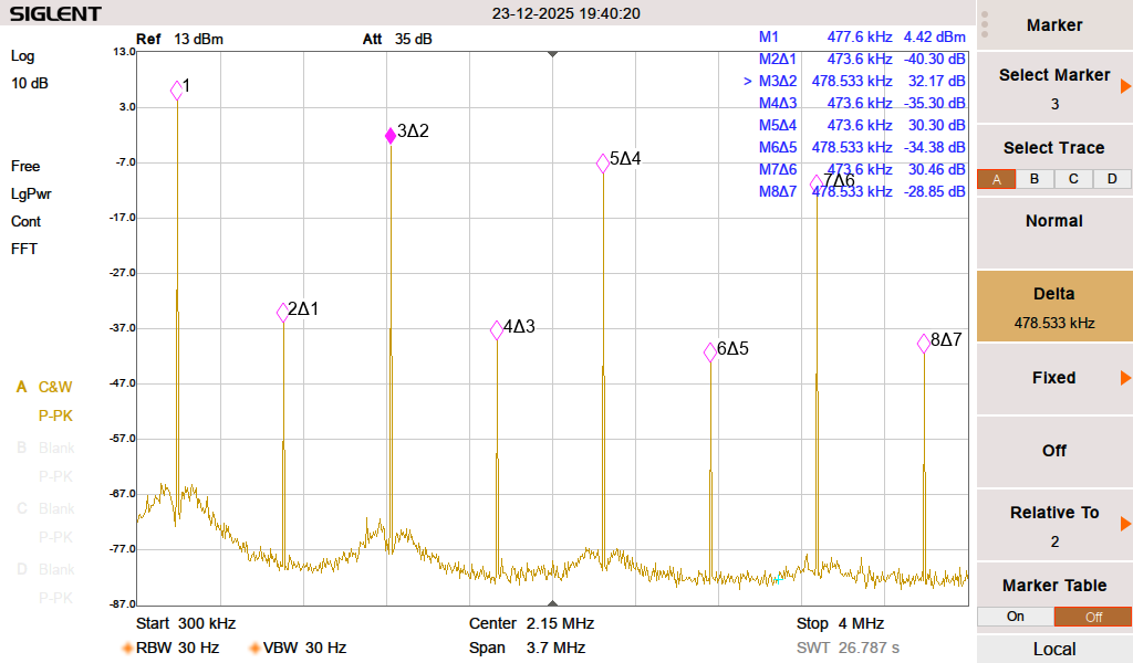
Definitely does not meet the out of band emissions standard set forth in FCC 97.307. Typical of solid state amplifiers, the odd harmonics are greater than the even.
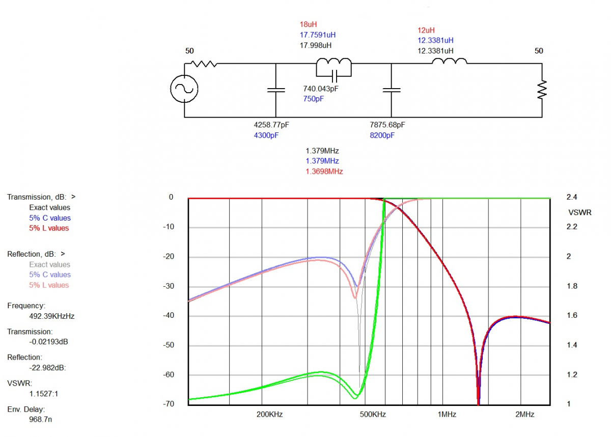
I used a filter design program called Elsie to design suitable filters for 630 Meters. There are two types of filters that can attenuate the harmonics; low pass and band pass. A low pass filter passes all emissions below the cutoff.
That is fine, however, it does not eliminate the possibility of interference and inter- modulation from frequencies below the band. Both types of filters are also good for receivers in the presence of AM broadcast band towers, which can desensitize receiver front ends when located nearby.
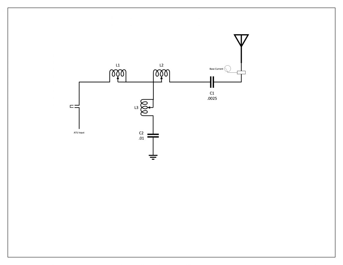
A band pass filter cuts off frequencies above and below the pass band.
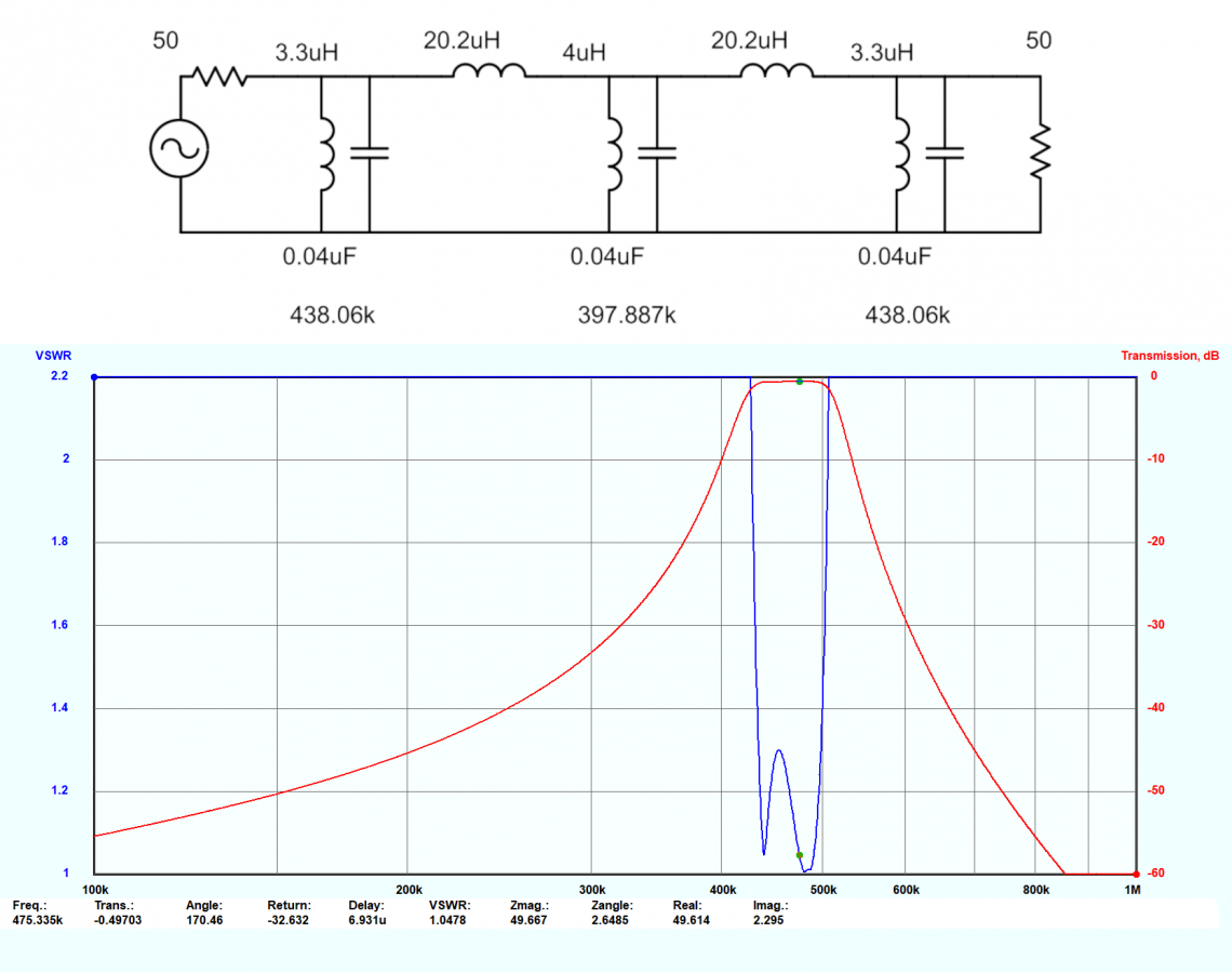
This is a nodal inductor-coupled band pass filter. I like this design because it has deep shoulders and has better performance with the harmonics in the AM broadcast band.
Prototype low pass filter:
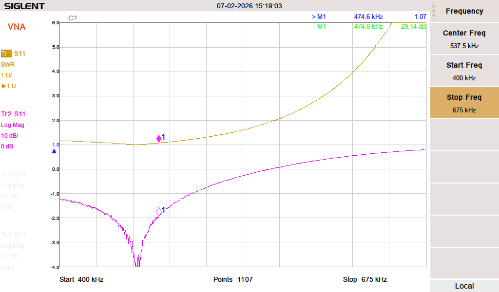
Quick prototype board. Capacitors are Cornell Dubilier silver mica dipped, the inductors are wound on T130-3 material. The SWR and return loss:
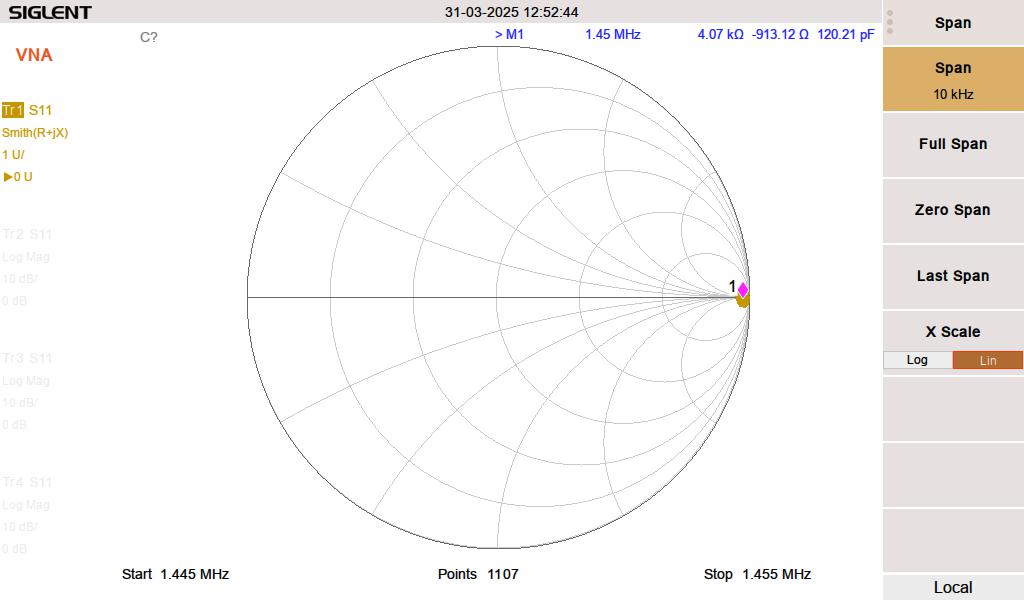
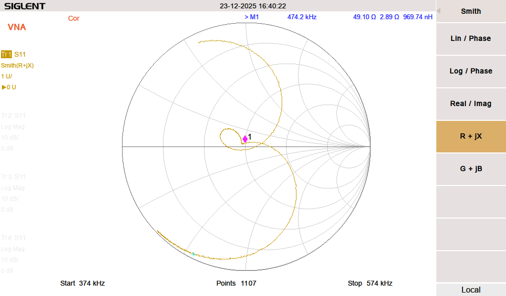
Smith chart:
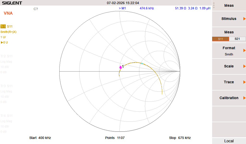
The Smith chart shows that it is slightly inductive on the desired frequency. The way to mitigate is to either add some capacitance (not easy) or reduce the inductance (somewhat easier). I tried tuning it by changing the spacing on the windings of L1 and L2. There was no change.
Low pass filter response:
The second harmonic on 951 KHz is -58.37 dBc. Harmonics 3 – 7 are 40 dB below the fundamental. This is adequate but the band pass filter below is better.
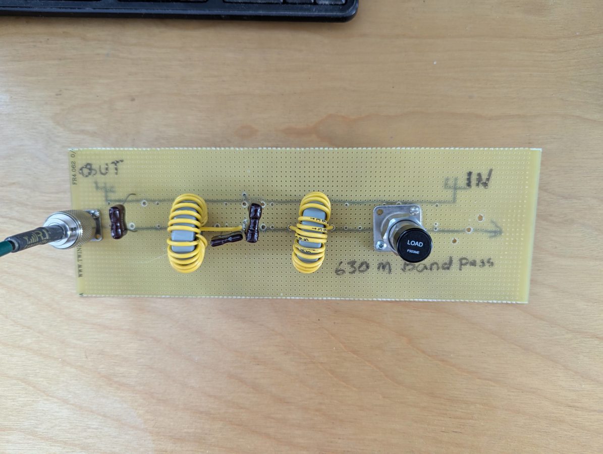
Prototype band pass filter:
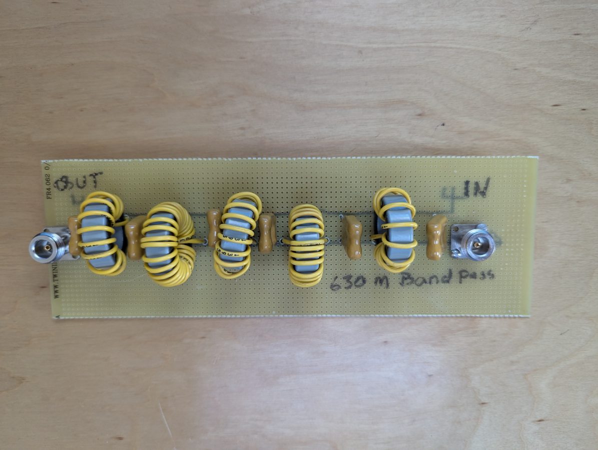
The above filter is a little rough, but it was a good test of the filter program’s design parameters. The capacitors are Cornell Dubilier 0.02 uF 500V. The inductors are wound on T130-3 iron powder toroid cores. The results are good:
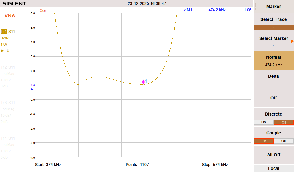
By adjusting the spacing of the windings on L3 (center of the board), I can tune the VSWR and Return loss for best values.
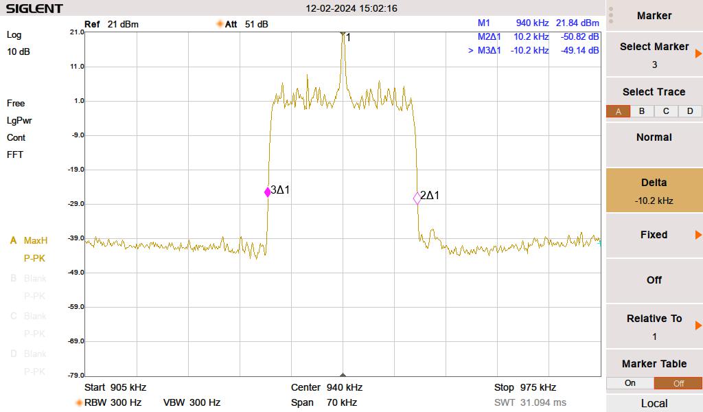
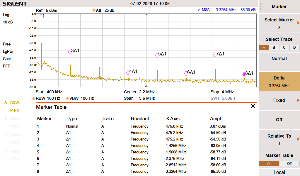
The same ZachTek WSPR transmitter noted above, running through the prototype filter:
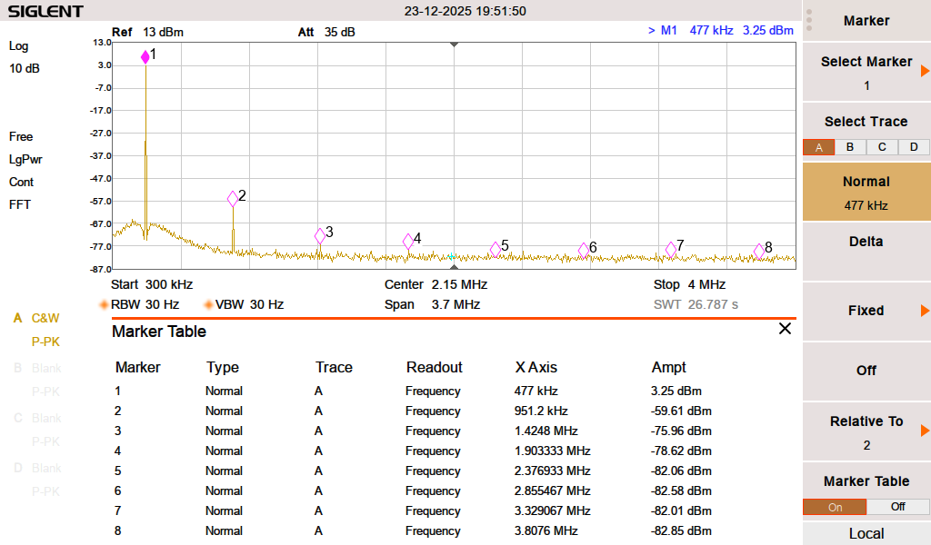
The second harmonic on 951 KHz is -62.86 dBc. The rest of the harmonics are less than that.
Of the two, the band pass filter has better performance characteristics. The return loss/SWR is lower and can be tuned by adjusting the spacing of the toroid windings on L3.
I decided to take the next step and make a PCB. I have KiCad on my Linux machine, which works well. Sometimes some of the foot prints need to be edited so the dimensions are correct, but that is easy.
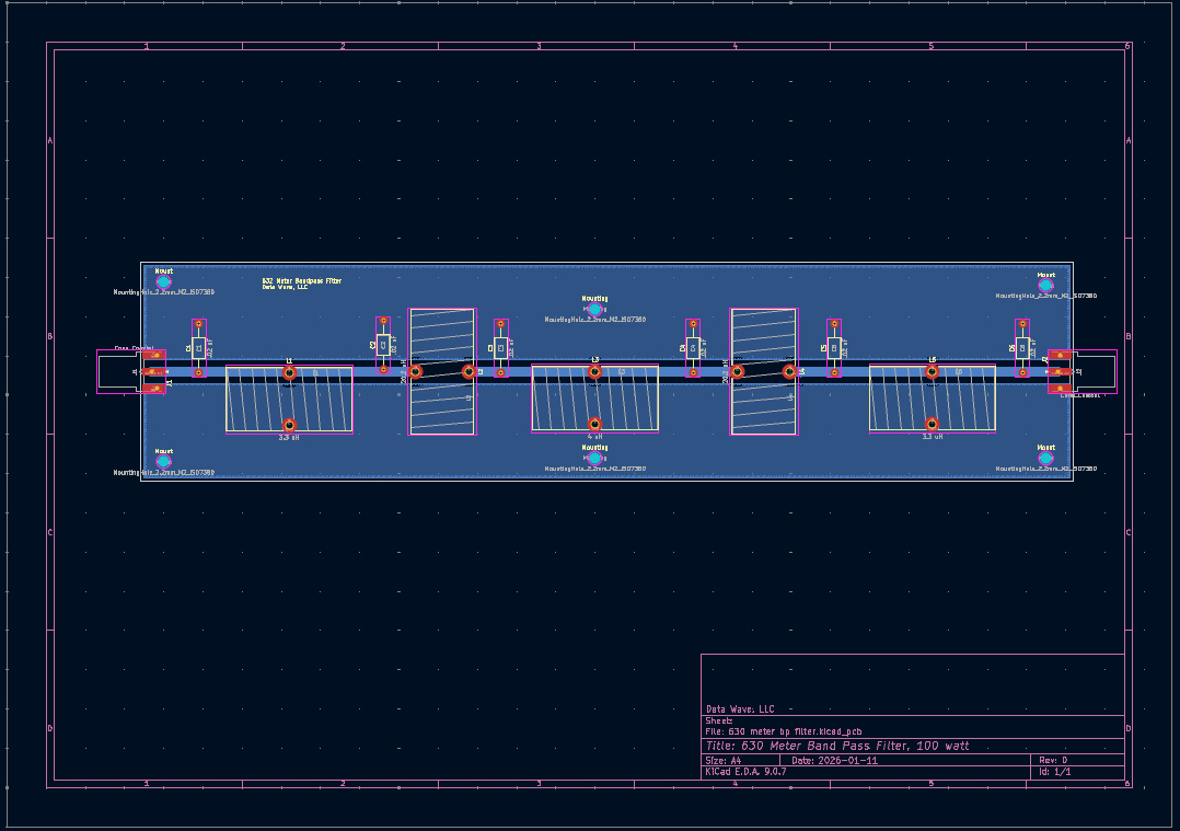
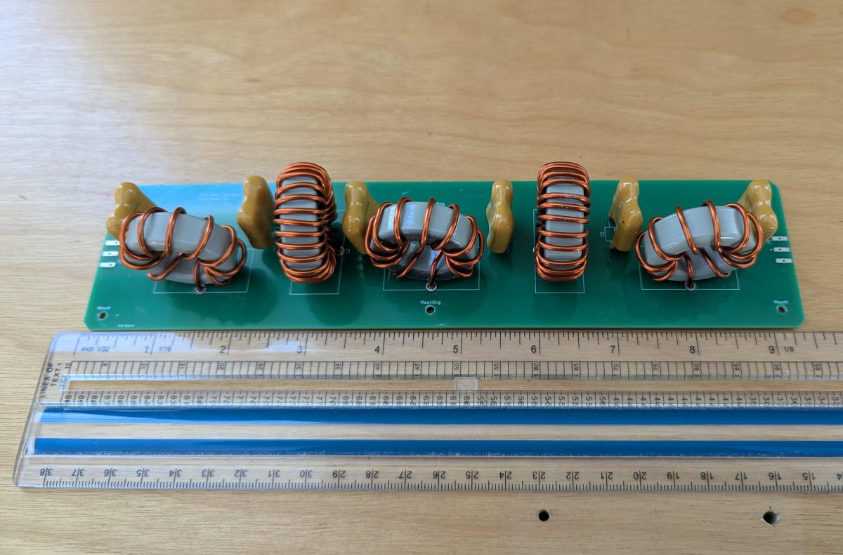
What I like about this board design is that it will work on any amateur band below 7 MHz with different component values. I had five boards fabricated and built one of them out. The T130-3 toroids are wound with 14 AWG magnet wire. The capacitors are same used in the prototype, 0.02 uF, 500V mica dipped.
Board mounted in aluminum enclosure:
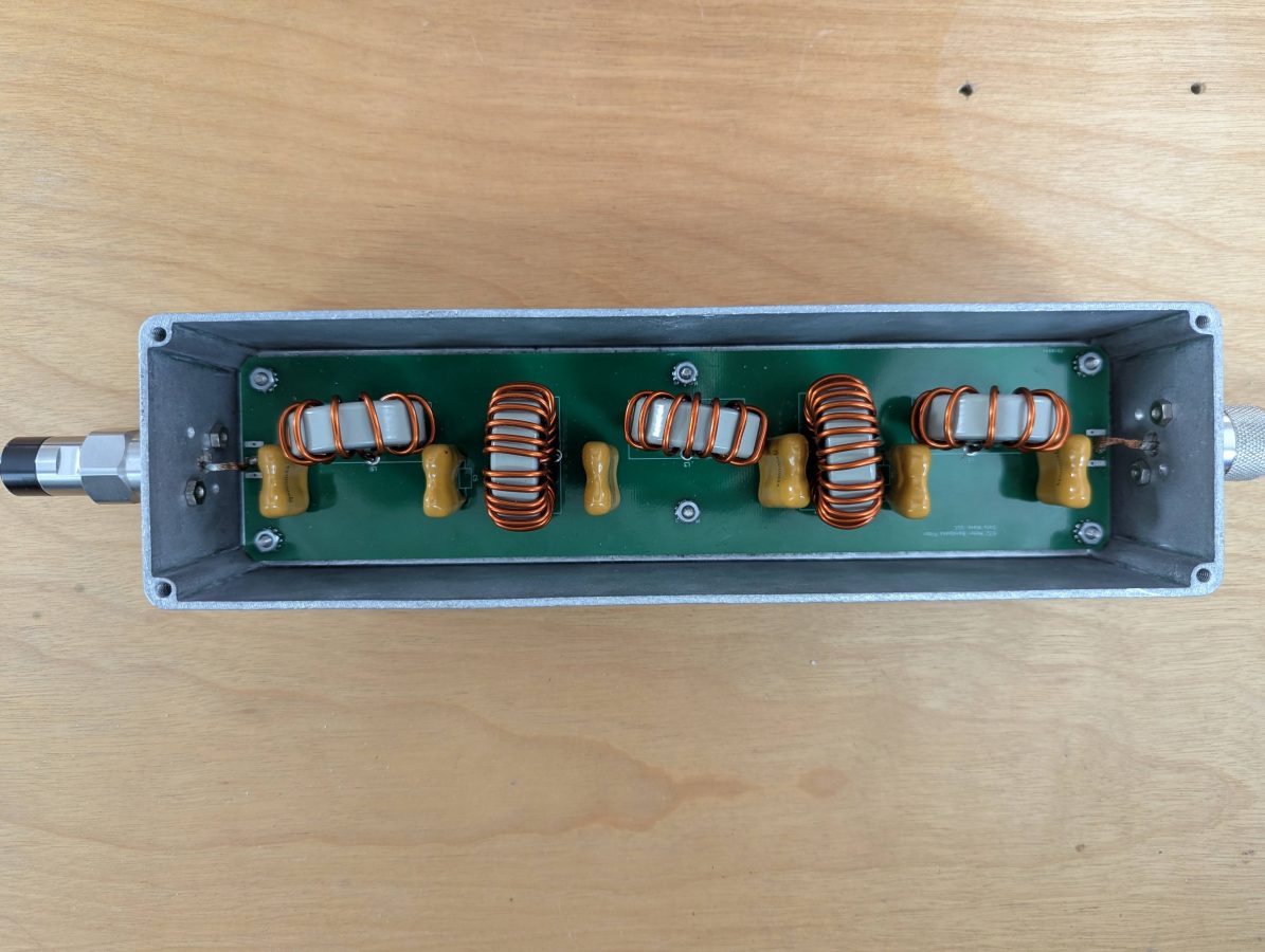
This build has similar measurements to the prototype board above. Based on what I found while making this, I made a few tweaks to the circuit board in KiCad. I would consider selling these, if there is enough interest.